Have you ever needed to sum only specific values in a range of data, and exclude others that did not meet the necessary criteria? The SUMIF Excel function and SUMIFS function enable you to do exactly this – sum values in a range of cells that meet specified criteria. Values that don’t meet the criteria are excluded from the sum.

SUMIF Function in Excel

The syntax for the Excel SUMIF function is as follows:

SUMIF(range, criteria, [sum_range])

It has these arguments:

range: range of cells to evaluate

criteria: number, expression, function etc. that indicates which cells should be added

sum_range: (optional) the cells to add, if different from “range”

Notes about SUMIF

The criteria can be a number, an expression, a function or a text string. The Excel SUMIF function restricts the data being summed according to a single criteria.

If the sum_range argument is omitted, the SUMIF function will assume that the sum_range is the same as the range.

One shortcoming of the SUMIF function in Excel is that it will only evaluate a single criteria, and in some situations that is not good enough. Microsoft thought of this situation and created another function, SUMIFS, to handle situations where multiple criteria must be evaluated:

SUMIFS Function in Excel

The SUMIFS function, unlike the SUMIF function, allows you to specify multiple criteria.  The syntax is:

SUMIFS(sum_range, criteria_range1, criteria1, [criteria_range2, criteria2], …)

the arguments to the function are:

sum_range: range of cells to add

criteria_range1: the range that is evaluated against criteria1

criteria1: number, expression, function etc. that indicates which cells in criteria_range 1 should be added

criteria_range2, criteria2: (optional) additional criteria and the corresponding range

Notes about SUMIFS

You may enter additional criteria as needed. While we can only use the Excel SUMIF function with one criteria, the SUMIFS function can be extended to handle 127 different pairs of criteria and criteria ranges.

Let’s take a look at an example that uses the Excel SUMIF function to solve an engineering problem.

Using the Excel SUMIF Function to Calculate a Sum Based on Criteria

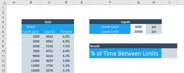
The worksheet shown below contains some measured stress in column B as well as the number of times the stress was at a certain level during the measurement period in column C.

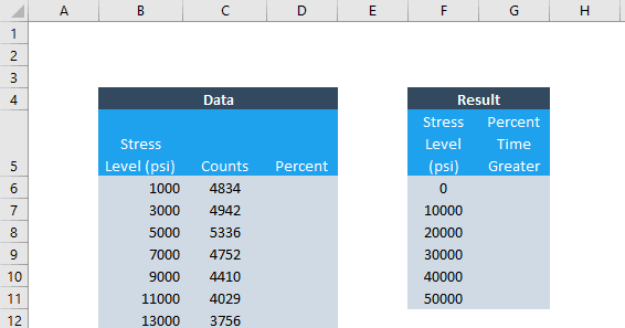
Create a column to calculate the percent of time at a stress level

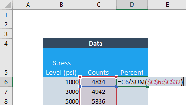
We will use the SUMIF function in Excel to calculate the percent of time that the stress was above a certain level. To do that, we’ll first calculate the percent of time represented by each count in column C. To do this, we’ll divide each count by the sum of all the counts.

Enter =C6/SUM($C$6:$C$3) in cell D6. If you prefer, you can select the cells with the mouse – remember to type F4 after you select the range for all the counts to create an absolute cell reference. This way the values in the denominator won’t change as we fill the formula into the rest of the column.

To fill the formula into the rest of the column, select cell D6 and double-click the fill handle.

Now column D displays the percentage of time that this location was at each stress level. In column G, use the Excel SUMIF function to calculate the percentage of time that the stress was greater than certain amounts.

Use the SUMIF function to calculate how often the stress exceeds a level

First, enter =SUMIF( in cell G6.

Remember, the syntax for the SUMIF function is SUMIF(range, criteria, [sum_range]).

The range to be evaluated is in column B, so select that range (click the first cell and type Ctrl-Shift-Down Arrow), then type F4 to make it an absolute cell reference.

So far, the SUMIF formula looks like this:

=SUMIF($B$6:$B$32

For the second argument in the SUMIF Excel function, we need to build the criteria.

Use the SUMIF Excel Function with inequality criteria

Use the concatenate function (&) to form a string joining together the greater than symbol (“>”) and the location of the cell that’s being compared (F6). Therefore, the second argument for the SUMIF function will be: “>”&F6.

It’s absolutely vital to include the quotation marks!

At this point the SUMIF formula will be:

=SUMIF($B$6:$B$32,”>”&F6

Again, add a comma after the argument.

For the final argument in the SUMIF function, select the sum_range, or the percent data in column D. Click cell D6, type Ctrl-Shift-Down Arrow, followed by F4. Add a close parenthesis to the SUMIF function. The final formula should be:

=SUMIF($B$6:$B$32,”>”&F6,$D$6:$D$32)

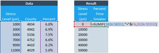
This formula tells Excel to check if the value in column B is greater than the value in column F, and if so SUMIF will sum the corresponding percentages from column D.

Type Enter, select the cell again, and double-click the fill handle. This is the resulting table:

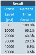
Examine the results of the Excel SUMIF function

It’s obvious from the data that the stress level is greater than zero 100% of the time. To check the other values resulting from the SUMIF formula, you can highlight the cells in column D that are greater than 10,000.

Excel will automatically display the sum of the highlighted cells in the lower left border of the window:

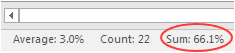
The sum should match the value calculated by the SUMIF Excel function.

Using SUMIFS to Calculate the Total Between Two Values

But what if we want to evaluate what percentage of the time the stress was between two values? We can add all the percentage values between the two limits shown on the worksheet below (6,000-20,000 psi), including the limits themselves.

Use the SUMIFS function when there are multiple criteria

To answer this question, we’ll solve using the SUMIFS function with two criteria, one for the lower limit and one for the upper limit. In the previous problem, we simply used the greater than (>) operator. In this example, we will include the limits in the criteria to see how to use the ≥ and ≤ operators in Excel.

The syntax for the SUMIFS function is as follows:

SUMIFS(sum_range, criteria_range1, criteria1, [criteria_range2, criteria2], …)

You’ll notice that the SUMIFS function has a different order for its arguments than the SUMIF formula. In the SUMIFS function, the range to be summed comes first. However, this argument is last (and optional) when using SUMIF.

Enter =SUMIFS( in cell K5. Select the percentages in column D.

Select the sum_range for the SUMIFS function

At this point, the formula will look like this:

=SUMIFS(D7:D33

Select the cell reference for criteria_range1

The second argument is the range of the first criteria. In this case, the criteria will be based on the stress in column B. At this point your formula should be:

=SUMIFS(D7:D33,B7:B33,

Set criteria1 for the SUMIFS function

The third argument, the first criteria, will be constructed similarly to the first example, but instead of “>” we will use “>=” which is Excel’s form of the ≥ (greater than or equal to) operator. Use & (ampersand) to concatenate to the cell containing the lower limit, G5.

=SUMIFS(D7:D33,B7:B33,”>=”&G5

That completes the first criteria.

Add the additional criteria to the SUMIFS function

We also need to add a criteria to limit the summed values for stress levels less than 20,000 (cell G6).

The SUMIFS function can take additional criteria by adding arguments for the range and criteria. This is something that the SUMIFS function can do that the SUMIF function cannot.

For this problem, the range will be the same. The criteria will simply be “<=”&G6, restricting the summed values to only those with a stress less than or equal to G6.

The final formula will be:

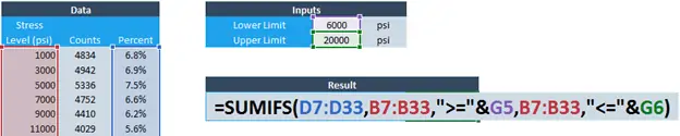
=SUMIFS(D7:D33,B7:B33,”>=”&G5,B7:B33,”<=”&G6)

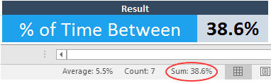
Again, we can quickly verify that this formula summed only the values that fall within the limits by highlighting the percentage values that correspond to stress between 6,000 and 20,000 psi. The value in the lower border should match:

You can adjust the limits in cells G5 and G6 and the SUMIFS function will update accordingly.

Errors with the SUMIF and SUMIFS Functions

SUMIFS #VALUE! Error

SUMIFS will return a #VALUE! error when the number of cells selected for criteria_range is different than the number of cells selected for sum_range. So if you are seeing this error, double check your cell references.

SUMIF and SUMIFS #REF Error

Either SUMIF or SUMIFS will return a #REF error if a cell reference has gone missing. This can occur if a column or row has been deleted from the spreadsheet. In this case, find the argument in the function that is returning #REF! and replace it with a new cell reference.

Wrapping Up

As you can see, the Excel SUMIF function and SUMIFS function allow you to sum only the values in a range of data that meet specific criteria. Use SUMIF when there is only a single criteria to evaluate, and SUMIFS when there are multiple criteria.

Here’s the syntax for the Excel SUMIF function one more time:

SUMIF(range, criteria, [sum_range])

And the SUMIFS function:

SUMIFS(sum_range, criteria_range1, criteria1, [criteria_range2, criteria2], …)

The example I’ve shown above is only one way to use these versatile functions. I’m sure you’ll encounter many ways to use SUMIF and SUMIFS in your projects as well!