Linear interpolation allows us to improve an estimate based on a set of x- and y-values. What if you are working with x-, y- and z-values, where x and y are independent variables and z is dependent on both? In that case, you can use bilinear interpolation in Excel. It works similarly to linear interpolation but uses a different formula.

As an example, let’s look at the following worksheet which contains air velocity data that is dependent on the horizontal position (x) and the vertical position (y).

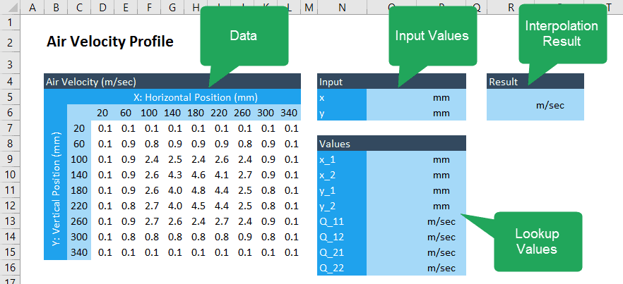
Setting Up the Worksheet

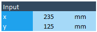
We can find an estimate of the air velocity for an x-value of 235 and a y-value of 125. Before we can start our bilinear interpolation in Excel, we’ll need to add these values into the sheet in the input section:

Elevate Your Engineering With Excel

Advance in Excel with engineering-focused training that equips you with the skills to streamline projects and accelerate your career.

Find Out More

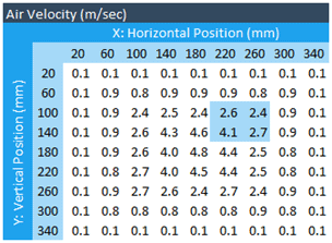
The z-value for x=235, y=125 will lie somewhere in between the highlighted values below:

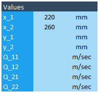
Named cells will make this worksheet much easier to work with. Remember, to name a cell or a range, simply select the desired cell(s), click in the name box to the left of the formula bar, and enter a name. Name the cell containing the x- and y-values you entered in x and y, respectively. Select the row of x-values in the data table and name those “xvalues”. Select the column of y-values in the same table and name those “yvalues”. Next, select all the air velocity numbers (cells D7-L15) and name them “zvalues”.

The formula for bilinear interpolation is:

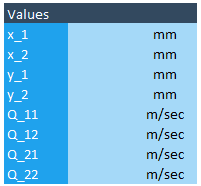
This is a complicated formula, but it can be broken down. We can use the INDEX and MATCH functions to find x₁, x₂, y₁, y₂, and the Q values to fill in this table:

Finding the x- and y-Values

First, we’ll focus on x₁ and x₂. The x₁ value is the value in the table that is just below our desired x-value of 235 (in this case, 220). The x₂ value is just above the desired value (in this case, 260). You can use INDEX and MATCH to find these values. This way, the spreadsheet will work for any x,y coordinates. In the box for x_1, enter the formula:

    =INDEX(xvalues,MATCH(x,xvalues,1))

The first argument tells the INDEX function to search within the xvalues array that was just defined. The position argument is the MATCH function. Here, the MATCH function searches for the value nearest to x (the name for the cell containing our desired x value) which doesn’t exceed it (because the last argument is 1). This function should return a value of 220 when you press Enter.

The formula for x_2 will be almost the same, so you can simply copy the formula into the cell for x_2. Edit the formula to add +1 at the end of the MATCH function:

    =INDEX(xvalues,MATCH(x,xvalues,1)+1)

This causes the position that INDEX looks in to be one more than the x_1 position. It should return a value of 260.

Now you have the x-values that are on either side of the lookup value of 235:

You can change the lookup value in cell O5 to verify that this works for any value within the range of x-values.

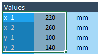
The formulas for y_1 and y_2 will be done in a similar fashion. For y_1, enter:

    =INDEX(yvalues,MATCH(y,yvalues,1))

For y_2, enter:

    =INDEX(yvalues,MATCH(y,yvalues,1)+1)

These should return values of 100 and 140 for y_1 and y_2, respectively.

To make the rest of your calculations easier, assign names to all of the cells in the Values table. Select the cells containing the names (x_1, x_2, etc.) as well as the cells containing the values.

In the Formulas tab, look in the Defined Names section. Click Create from Selection. Make sure the Left Column checkbox is clicked in the box that appears. This will automatically apply the names from the left column to the cells on the right.

Look Up the Q-Values

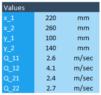
To fill out the rest of the Values table, we’ll need to find the Q values. The Q values are actually z-values (the dependent variable in the middle of the air velocity data table). Q₁₁ is the z-value that corresponds to x₁ and y₁; in this example, that would be 2.6 (the value found underneath 220 and to the right of 100). Q₁₂ is the z-value that corresponds to x₁ and y₂ (4.1 in this example) and so on.

You may recall that the INDEX function can be used to look up data in a two-dimensional data table. For reference, its syntax is:

INDEX(array, row_num, [col_num))

It has arguments for both vertical position (row_num) and horizontal position (col_num). We’ll use both of those arguments to extract z-values from the data table. Both arguments will use the MATCH function to select the position. Begin the function by looking in the zvalues array:

    =INDEX(zvalues

The row number will be determined by doing a lookup with MATCH on the yvalues array. We will be looking for y_1, which is an exact position on the table, rather than a value in between the given values. Therefore, we’ll be looking for an exact match to y_1, and the last argument of the MATCH function will be 0.

    =INDEX(zvalues,MATCH(y_1,yvalues,0)

The last argument for INDEX will be the column number. This will be a lookup for the exact value of x_1 within the xvalues array:

    =INDEX(zvalues,MATCH(y_1,yvalues,0),MATCH(x_1,xvalues,0))

Just to review, the first argument tells INDEX what array to look in (the z-values array). The second argument tells INDEX the vertical position in the z-values array (with an exact match to y_1). The third argument tells INDEX the horizontal position (with an exact match to x_1). This formula should return a value of 2.6, because that’s the value you’ll find in the table when you look below 220 (x_1) and to the right of 100 (y_1).

The rest of the Q values can be found in a similar fashion. You can copy the formula for Q_11 and edit it to match these formulas:

Q_12:     =INDEX(zvalues,MATCH(y_2,yvalues,0),MATCH(x_1,xvalues,0))

Q_21:     =INDEX(zvalues,MATCH(y_1,yvalues,0),MATCH(x_2,xvalues,0))

Q_22:     =INDEX(zvalues,MATCH(y_2,yvalues,0),MATCH(x_2,xvalues,0))

Add names to those cells by selecting the cell with the name and the value. In the Formulas tab, go to the Defined Names section, then click Create from Selection. Click OK in the box that appears. The completed table should look like this:

Bilinear Interpolation in Excel

The only step that remains is to enter the formula for bilinear interpolation in Excel notation. Click within the result cell and enter:

=1/((x_2-x_1)*(y_2-y_1))*(Q_11*(x_2-x)*(y_2-y)+Q_21*(x-x_1)*(y_2-y)+Q_12*(x_2-x)*(y-y_1)+Q_22*(x-x_1)*(y-y_1))

The result is 3.2 m/s. We can check to see if this result makes sense by referring to the data table. You’ll see that it falls within the area that’s highlighted in the table in the beginning of the section.

Validating the Interpolation Result

One way to check that the formula is working correctly is to use an x-value that’s exactly in the middle between 220 and 260, and a y-value that’s exactly in between 100 and 140. Enter 240 for x and 120 for y.

The result should be the average of those four highlighted cells (simply select the cell to see the average in the bottom of the Excel window):

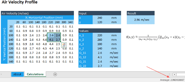
The result does match the average (shown with a red arrow). (You can increase the decimal places shown on the result cell by clicking the button in the Number section of the Home tab.)

Another method of validation is to enter values that are very close to x- and y-values in the chart, for example 220.1 and 100.1. This should give you a result of 2.61, which is very near the z-value that corresponds to those x- and y- values.

Wrap-Up

Bilinear interpolation in Excel is made possible by the INDEX and MATCH functions. I use it a lot to improve the accuracy of my calculations, and now that you know how to use it, I’m sure you will too.