You can use Excel to fit simple or even complex equations to data with just a few steps.
Determine the Form of the Equation
The first step in fitting an equation to data is to determine what form the equation should have. Sometimes this is easy, but other times it will be more difficult. Usually, the equation you choose will come from prior knowledge of the system you are analyzing.
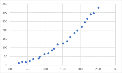
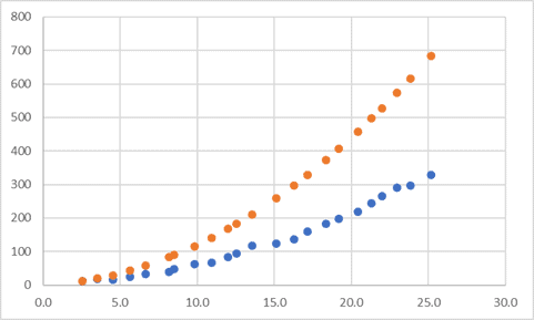
Either way, it all starts with inspecting the data, and the easiest way to do that is to plot it in a chart. I’ve done that with some sample data below, and it’s obvious that we can fit a quadratic function to this data. Regardless of the complexity of the function, the method I’ll be showing is still valid. I’ve just chosen a simple example for this demonstration.
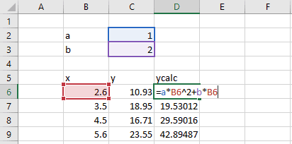
Once you’ve determined the form the equation should have, the next step is to define the parameters for the equation. Assuming the y-intercept is 0, a quadratic equation has the form:

Elevate Your Engineering With Excel
Advance in Excel with engineering-focused training that equips you with the skills to streamline projects and accelerate your career.
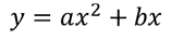
so, our parameters are a and b.
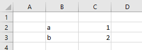
We can input arbitrary values for those parameters on our spreadsheet. The values that are entered don’t matter for now because we’ll be adjusting them later to fit the function to the data.
Calculate the Equation from the Parameters
Next, we calculate a new series in Excel using the equation above. The series will be a function of the parameters a and b, and the independent variable, x.
Plotting the original y-data and the calculated result, “ycalc”, on the same graph tells us that the parameters of the function are not yet correct. But we will fix that soon by adjusting them to find the best fit.
Calculate the Sum of Residuals Squared
Although it would be tedious, we could manually adjust the two parameters and “eyeball” the curve fit until it looked good. But we’re smarter than that, so we’ll use the method of least squares along with Solver to automatically find the parameters that define the best fit curve much more efficiently.
Solver works by optimizing a single objective cell, so we’ll need to create an output that defines how well the function fits the data. This output is the sum of the residuals squared.
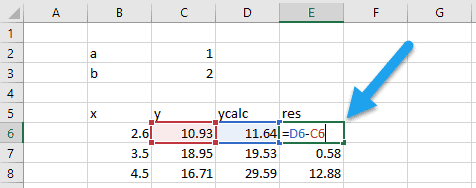
Residuals are the difference between the value provided by the function and the data value at a given value of x.
So, let’s create another column for the residuals:
Then, to calculate the sum of the residuals squared, use the SUMSQ function:
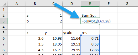
Minimizing this term will let us know that we have found the parameters that best fit the function to the data. To minimize this term, we’ll use Solver.
Find the Best-Fit Parameters
If you haven’t already activated the Solver add-in in your copy of Excel, you can find instructions to do that right here.
Once installed, you can open it from the far-right side of the Data tab:

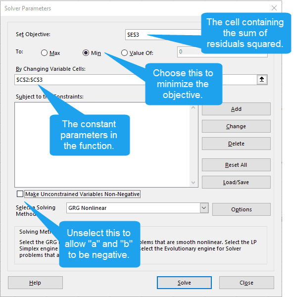
With Solver open, select the cell that contains the SUMSQ formula as the objective, and the cells containing the values for “a” and “b” as the variable cells.
The goal, of course, is to minimize the sum of the residuals squared, so select the button next to “Min” in the Solver window.
Finally, uncheck the box next to “Make unconstrained variables non-negative.” We don’t know beforehand that the best values of a and b are necessarily positive, so this constraint is invalid.
For my worksheet, the Solver window has the following setup:
For a simple model like this, it’s not necessary to change any of the solver options. However, for more complex equations that may be necessary, and I’ve explained how to do so in this post.
All that’s left now is to click “Solve” and let Solver find the optimum parameters for the function.
Check the Result
Solver adjusts the values of the constants until the sum of the squared residuals is minimized. Those values are shown below:
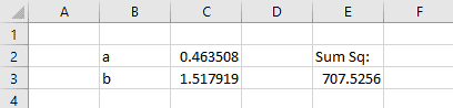
The magnitude of the minimized sum of squared residuals is relative and depends on the data you are working with. Smaller data values are going to result in a smaller sum of squared residuals than larger values.
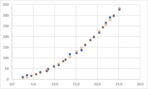
Finally, we can check the fit of the equation to the data by plotting both on the same chart. In the chart below, the orange circles are the function and the blue circles are the underlying data from which the function was derived.