
Recently I wrote about linear interpolation in Excel and showed how to do this in a worksheet. In this post, I’ll show you how to wrap this entire process into a linear interpolation VBA function. This is an essential function to keep in your toolbox if you find yourself needing to interpolate from tables of data frequently. Since I’ve created this function for my own worksheets, I’ve been surprised at the number of times that I’ve used it myself.
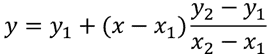
The code and the math are straightforward. We’ll need to gather the input values and estimate the value of y using the following equation:
Create the Linear Interpolation VBA Function
With the VBA editor open, insert a module into the workbook by right-clicking on the workbook in the project window and selecting Insert>Module. Adding the module automatically opens a new code window.

Elevate Your Engineering With Excel
Advance in Excel with engineering-focused training that equips you with the skills to streamline projects and accelerate your career.
We’ll need to give the function a name – I’ll call it “LinInterp”.
To perform the calculations, three arguments are required:
- The value of x for which we want to estimate a corresponding y-value.
- An array of known x-values
- An array of known y-values
So we’ll enter those arguments, separated by commas. The first line of the function should look like this:
Function LinInterp(x, xvalues, yvalues)
Excel automatically adds the last line “End Function” when you type enter after the first line.
Gather the Inputs
According to the linear interpolation equation, to estimate y, we’ll need to gather a few values from our table of x- and y-data: x1, y1, x2, and y2.
We can use INDEX and MATCH to pull the values from the spreadsheet into the linear interpolation VBA function, but there’s a catch.
VBA doesn’t recognize these functions by themselves. In order to use them in our function, we have to tell VBA that they are worksheet functions. We can do that by preceding the function name with “Application.WorksheetFunction”.
So the line of code that extracts the x1 value from the table looks like this:
x1 = Application.WorksheetFunction.Index(xvalues, Application.WorksheetFunction.Match(x, xvalues, 1))
We’re telling VBA to look in the array of “xvalues” and find the position largest value that is less than x with the MATCH function, then return the value of x in that position and assign it to the variable x1.
Of course, this assumes that the values of x are in ascending order from top to bottom.
To find x2, we’ll use essentially the same function. But instead of finding the position of the largest value that is less than x, we’ll add 1 to that position to get the position of the next value that is greater than x.
The formula looks like this:
x2 = Application.WorksheetFunction.Index(xvalues, Application.WorksheetFunction.Match(x, xvalues, 1) + 1)
Similarly, we’ll get the values of y1 and y2 with these formulas:
y1 = Application.WorksheetFunction.Index(yvalues, Application.WorksheetFunction.Match(x, xvalues, 1))
y2 = Application.WorksheetFunction.Index(yvalues, Application.WorksheetFunction.Match(x, xvalues, 1) + 1)
Calculate the Output
Finally, with all of the inputs gathered, we can estimate the value of y.
LinInterp = y1 + (y2 – y1) * (x – x1) / (x2 – x1)
Notice that the equation does not start with “y =”. We need to match the name of the function here, so that something can be returned to the spreadsheet when we call the function.
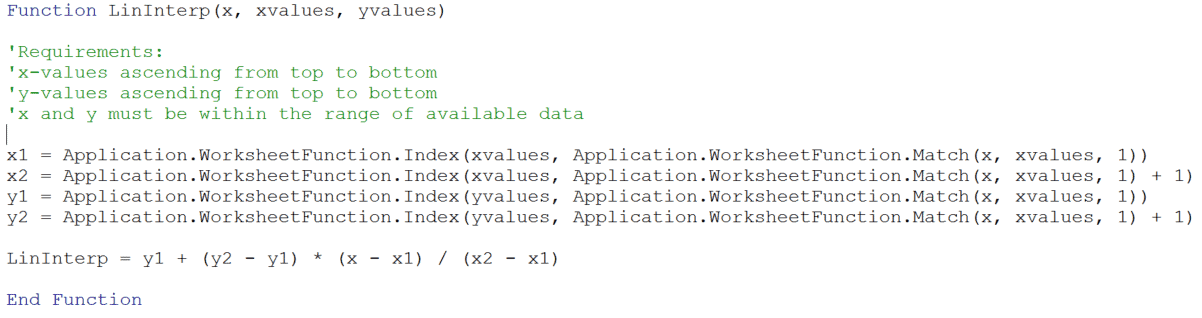
The completed function should look like this (I’ve also added a few comments to identify some of the shortcomings of this simple code):
Testing it Out
To make sure it’s working as expected, let’s test it out. I’ll use the same data from my previous linear interpolation post – air density vs. temperature. The data is tabulated for every 20 degrees C from 0 to 100.
Let’s try to use the function to estimate the air density at 50 C.
When I start typing the name, Excel recognizes it as a function and auto-suggests it, just like a built-in function.
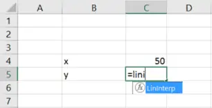
With the function name highlighted in the tooltip window, typing Tab automatically adds the function to the cell.
Next, select the arguments for x, xvalues, and yvalues:
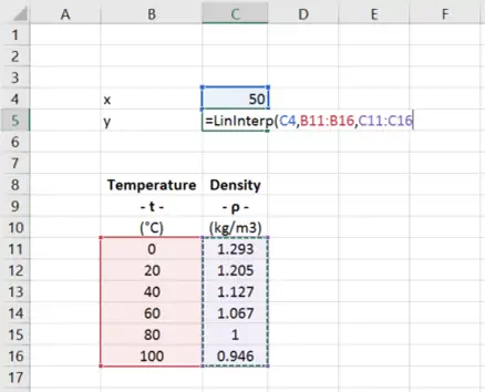
Type Enter, and the function returns the y-value: 1.097.
To check that this value indeed makes sense, we can plot it on a scatter chart with all of the temperature and density data:
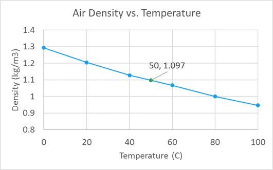
The x-y pair lies exactly on the line connecting the densities at 40 and 60 degrees C, so we can be confident that the linear interpolation VBA function is returning a correct value.