

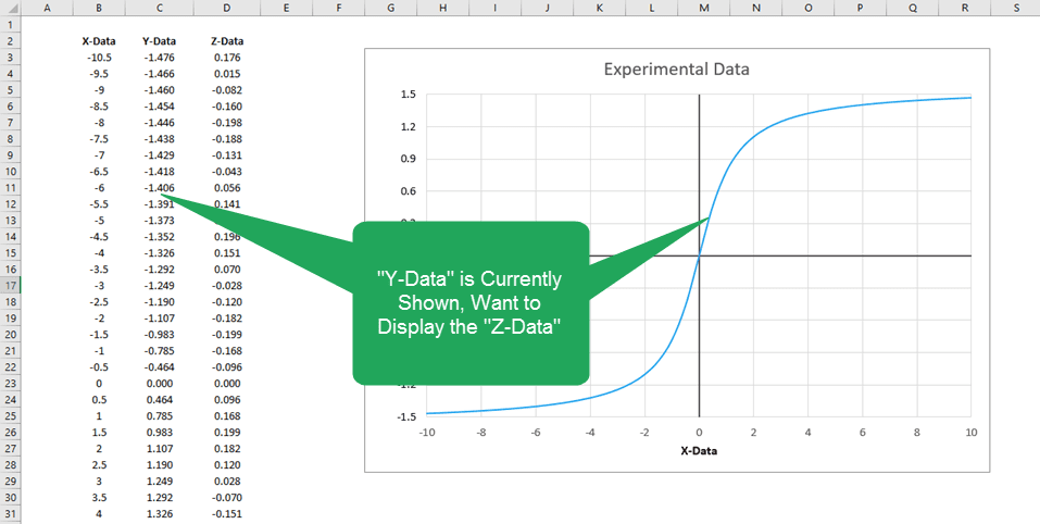
At some point, you’ll probably need to update a scatter chart in Excel. Perhaps you’ll need to import new data, but in some cases the new data is already contained in the worksheet. In this example, the data from column C has been plotted, but there’s an additional column of data in column D that needs to be plotted. I’ll show you three different ways to change the chart to use the new column of “Z-data” instead of the old data. A scatter chart is shown here, but the same concepts could be applied to a bar, column, or line chart too.
Method 1: Select Data Source Window

Elevate Your Engineering With Excel
Advance in Excel with engineering-focused training that equips you with the skills to streamline projects and accelerate your career.
This first method is one you may have used before: just right-click anywhere in the chart area and choose Select Data.
The Select Data Source window will appear:
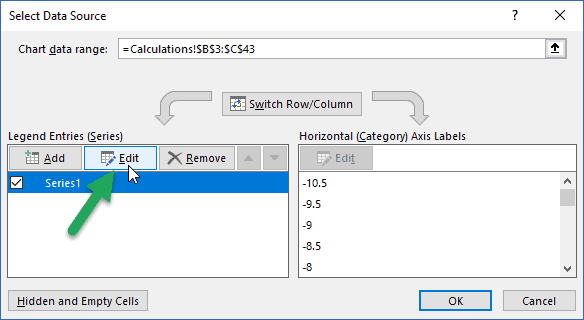
Note that the Chart data range contains the B and C column ranges, and that the chart contains one series, shown in the box at lower left.
Click the Edit button just above that series to edit the input data.
You may enter a Series name by clicking inside the first box, then selecting the header for Column D, but this is optional.
The X values should remain the same. To edit the Y values, select the entry in the third box, and delete it.
Select the new data (click in cell D3 and drag down to the end of the column) and click OK.
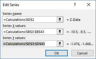
In the Select Data Source window, you’ll see that the series has been updated with the new name from cell D2.
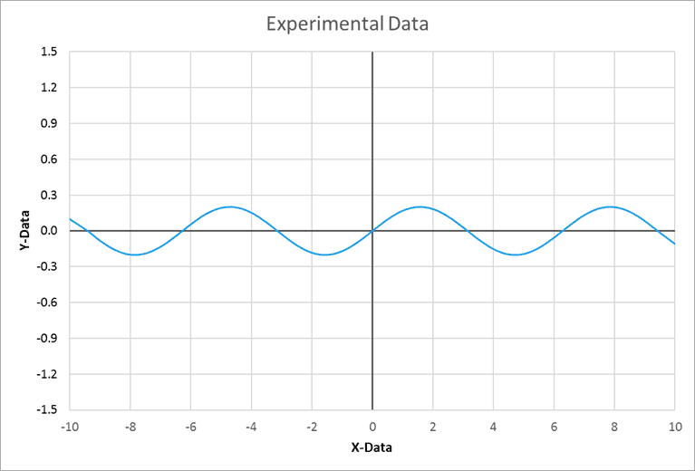
Click OK again, and the new data will be included in the chart. In this case, it’s a sine wave.
Method 2: Click and Drag to Update a Scatter Chart in Excel
Another method to use is to left-click on the data displayed in the chart. The data columns for the curve will become highlighted.
Hover the mouse over the border of the Y Data until the mouse pointer changes to a pointer with four arrows:
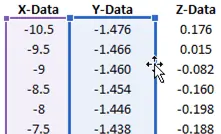
Click and drag over to the Z-Data column. This will move the selection, and the chart will update.
Method 3: Formula Bar
The final way to update a scatter chart in Excel is through the formula bar. Left-click on the curve in the chart. If you look at the formula bar, you’ll see it’s referencing column B for the X data and column C for the Y data:
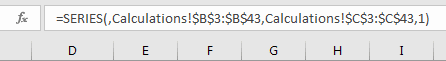
Simply change the “C”s to “D”s and the chart will update accordingly.
I rely on this method often, especially when I need to update the number of rows of data included in a chart. It’s much quicker to update the reference in the formula bar than to click and drag all the way to the bottom of a long column of data.
Wrap Up
There you have it: three distinct ways to update a scatter chart in Excel. You’ll probably find, like I have, that the second and third methods can save a ton of time over using the Select Data Source method. Over a year’s work, the time savings can amount to hours of effort!