
You saw in the pressure drop example that LINEST can be used to find the best fit between a single array of y-values and multiple arrays of x-values. In that example, we raised the x-values to the first and second power, essentially creating two arrays of x-values. That characteristic allows LINEST to do multiple linear regression, where there are several different arrays of independent variables and a known output.
Our worksheet contains measurements of escaping hydrocarbon mass during an operation where gasoline is pumped into a tank. The data set contains measurements of tank temperature, gasoline temperature, initial tank pressure, and the gasoline pressure. Assuming that the mass of escaping hydrocarbons is a function of the other four variables, we can predict the amount of escaping hydrocarbons for a given set of the independent variables. LINEST can be used to find coefficients for each of the variables.
The worksheet contains space for the four variable coefficients plus a constant. Select those five cells, then go to the formula bar and begin the array formula:
=LINEST(
The known y’s are the masses of escaping hydrocarbons.
=LINEST(F6:F37,

Elevate Your Engineering With Excel
Advance in Excel with engineering-focused training that equips you with the skills to streamline projects and accelerate your career.
There are multiple known x-arrays, so for the second argument, select all of the other columns of data: tank temperature, gasoline temperature, initial tank pressure, and gasoline pressure.
=LINEST(F6:F37,B6:E37,
The third argument will be TRUE so that LINEST can calculate the constant. We have no reason to assume there wouldn’t be a constant for this problem. The fourth argument will be FALSE to omit regression statistics.
=LINEST(F6:F37,B6:E37,TRUE,FALSE)
Since it’s an array formula, type Ctrl-Shift-Enter. LINEST will output coefficients for each input variable. However, please note that LINEST returns the coefficients in the opposite order of the input columns. Gasoline pressure is the first coefficient to be returned, but it was the last column in the data. This is somewhat counterintuitive, so try to remember that LINEST works this way when you use multiple x arrays.
To see how well the regression worked, add a column to the right of the data table labeled Prediction (grams). We’ll calculate the prediction by multiplying each variable by its coefficient, then summing those products.
=I6*E6+J6*D6+K6*C6+L6*B6+M6
Since this formula will be copied into the rest of the column, the coefficients all need to be absolute cell references. Click within each coefficient (I6, J6, K6, L6 and M6) and press F4. Your formula should now be:
=$I$6*E6+$J$6*D6+$K$6*C6+$L$6*B6+$M$6
Press Enter, then double-click the fill handle to fill the formula into the rest of the column.
To check how well the prediction fits the measured values, we can plot them against each other. Select the Hydrocarbons Escaping column and the Prediction column and create an XY scatter chart.
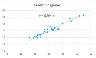
Ideally, if all of the data fit the equation just perfectly, a linear trendline for this plot would have a slope of 1. Add a linear trendline and set the y-intercept to zero. Display the equation on the chart to see the slope. In this case, the slope is 0.994, which is quite close to 1. This tells us the calculated values are matching the measured values at almost a 1:1 ratio on average. The scatter in the data is shifting the slope slightly, but that’s to be expected when fitting a line to measured data. Overall, the multiple linear regression gave a satisfactory fit.